

- Published on
Exploring GPT-3: A Comprehensive Illustrative Guide to the AI Behind ChatGPT (Part 1)

Table of Contents
- Introduction
- Datasets used to train GPT-3
- Pre-Processing/Cleaning/Filtering the Datasets
- Tokenization: For creating a dictionary of tokens/vocabulary to index tokens
- Embedding: Converting tokens to a vector of floating numbers
- Summary So far
- Model’s Architecture
- OpenAI GPT’s Working through Illustrations
- Training Details of the Model
Introduction
GPT-3 is a phenomenal thing that has happened in NLP history. For the first time ever, people are able to see Large Language Models (LLMs) generating human-like text (publicly). The fact that GPT-3 is able to generate text that is incredibly difficult to distinguish whether it is written by a human or an AI is an incredible feat to achieve.
Before diving into the details, here’s the outline of the entire blog we’re going to journey through to understand the working principles of GPT-3.
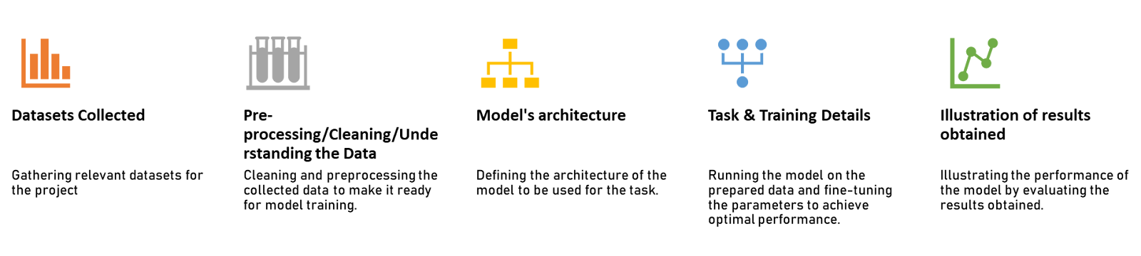
Figure: Flow diagram indicating the process of understanding a machine learning task.
Datasets used to train GPT-3
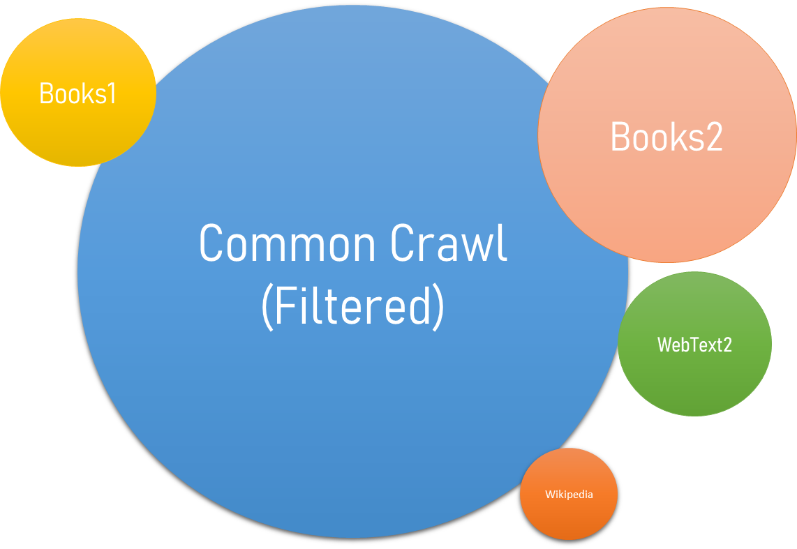
Datasets for language models have rapidly expanded, culminating in the Common Crawl dataset constituting nearly a trillion words.
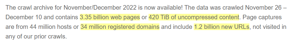
Figure: Common Crawl’s latest crawled data (November/December 2022)
Fact: Google also crawls the entire world wide web to train their search engines but they do not publish them publicly as Common Crawl does.
What is WebText2?
Here’s what OpenAI mentioned about WebText in their GPT-2 research paper:
“Manually filtering a full web scrape would be exceptionally expensive so as a starting point, we scraped all outbound links from Reddit, a social media platform, which received at least 3 karma. The resulting dataset, WebText, contains the text subset of these 45 million links. … contains slightly over 8 million documents for a total of 40 GB of text.”
WebText2 is an extension of WebText with more links, documents, and huge gigabytes of text. OpenAI hasn’t publicly released WebText Dataset but we have a replica named “Openwebtext2” available to everyone with which you can experiment and probably train your innovative model with it.

Though, it’s not really useful for ordinary people to know about these gigantic datasets. Since in reality, a normal developer cannot have the resources and infrastructure that could store these and train the models. But the concepts behind pre-processing/cleaning/filtering them is something worth giving attention to.
So, the above theory is just a theory, not anything to ponder upon.
Pre-Processing/Cleaning/Filtering the Datasets
Task 1: Improve the Quality of the Datasets collected
They have done three things to improve the quality of the datasets
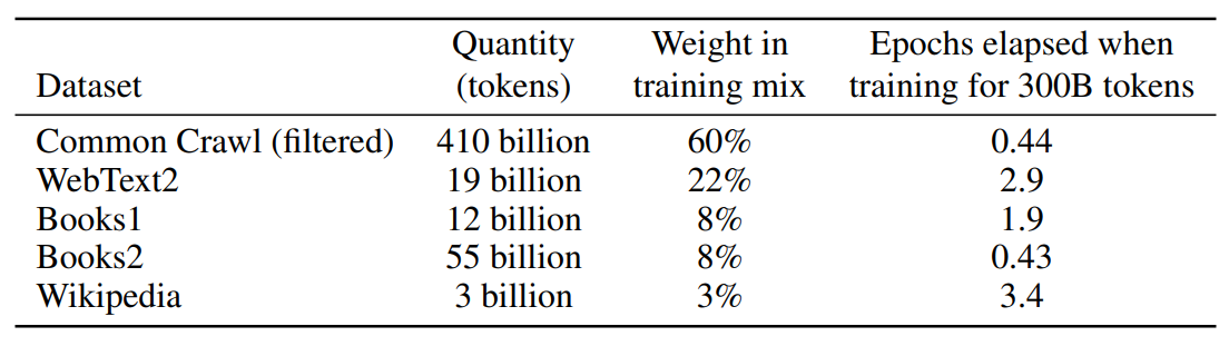
- Filtered a version of CommonCrawl based on similarity to a range of high-quality reference corpora
- Performed fuzzy deduplication at the document level, within and across datasets, to prevent redundancy and preserve the integrity of our held-out validation set as an accurate measure of overfitting
- Added known high-quality reference corpora (WebText2, Books1, Books2, Wikipedia) to the training mix to augment CommonCrawl and increase its diversity.
The Interesting thing to note here is that to understand both points 1 and 2 we need another blog post. And also it is important to understand that no matter how brilliant your model is if you don’t give proper attention to filtering, and splitting your dataset properly into train, test, and validation sets without any overlapping (data contamination), your efforts will go in vain. So understanding and working with the dataset should be anyone’s first priority over the model’s architecture. That’s the reason for the above three additional steps being applied for improving the quality of the datasets.

Figure: Picture depicting the importance of handling the dataset over the model’s architecture
Pause now and think about what we should do next (we’ve discussed the cleaning part up to now). At a very broad level, if you think about what we should do next after cleaning, and filtering the dataset we need to do two things:
Tokenization: For creating a dictionary of tokens/vocabulary to index tokens
So, we need to form a vocabulary of tokens and OpenAI GPT uses a data compression algorithm which is Byte-pair encoding(BPE) algorithm for this purpose. This comes under the category of sub-word (not necessarily a character or a word) tokenization.
Do not ignore the upcoming point! This is really something big to give your full attention to. The answer to the question “How we can process/tokenize a document containing text which is made of words at a broad level or of characters at a subtle level?” is damn important to find out.
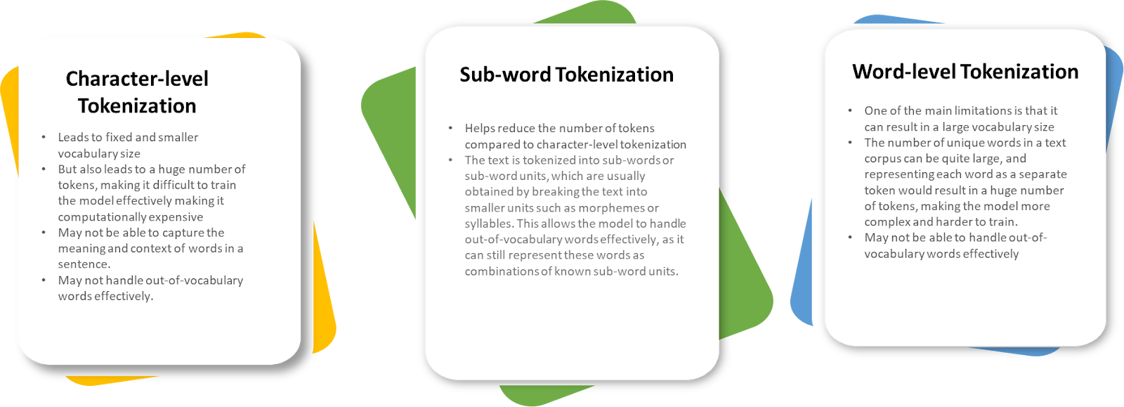
There are different types of Tokenization techniques available like word level, sub-word level, character level, sentence level, regex-based, n-gram tokenizations, etc… However, we just need to understand the three most frequently used tokenization techniques. Here’s an illustration of that.
Words are boring but illustrations and practical demonstrations are interesting, correct? Let’s learn more about the sub-word Tokenization through an illustration with the freely available OpenAI tokenizer. Try it out if you want to!
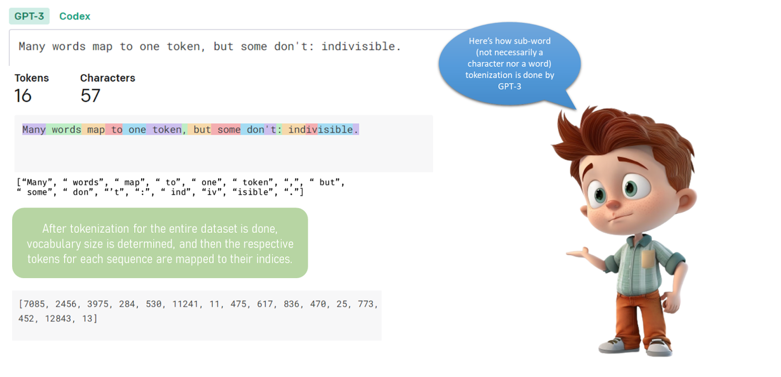
“A helpful rule of thumb is that one token generally corresponds to ~4 characters of text for common English text. This translates to roughly ¾ of a word (so 100 tokens ~= 75 words).” (Source)
If you think “Why can’t I divide this into word-level tokens where each token is a word?” the answer is fairly simple. It makes vocabulary size grow along with the dataset. Digging into more detail, having word-level tokens vocabulary is never a good idea. Since we can have thousands to millions of unique words in huge datasets, this means we should have 1 million neurons (let’s vocabulary size is 1 million) in the output layer to predict the next word given a sequence of words which is computationally expensive. In other words, if the model needs to predict the next word it has to look up the entire 1 million words to find the next word!!
InEffective Out-of-Vocabulary(OOV) words Handling: Additionally, the model struggles with words that are not part of its vocabulary, meaning that if an unknown word is encountered, it is often unable to tokenize it into constituent words that are in the vocabulary.
One sentence explanation for the choice of the tokenization algorithm is, we have to make a trade-off between the vocabulary size and the number of tokens along with effective handling of out-of-vocabulary tokens and sub-word level tokenization is the best choice for that. Note that character-level tokenization leads to a huge number of tokens and less generalization.
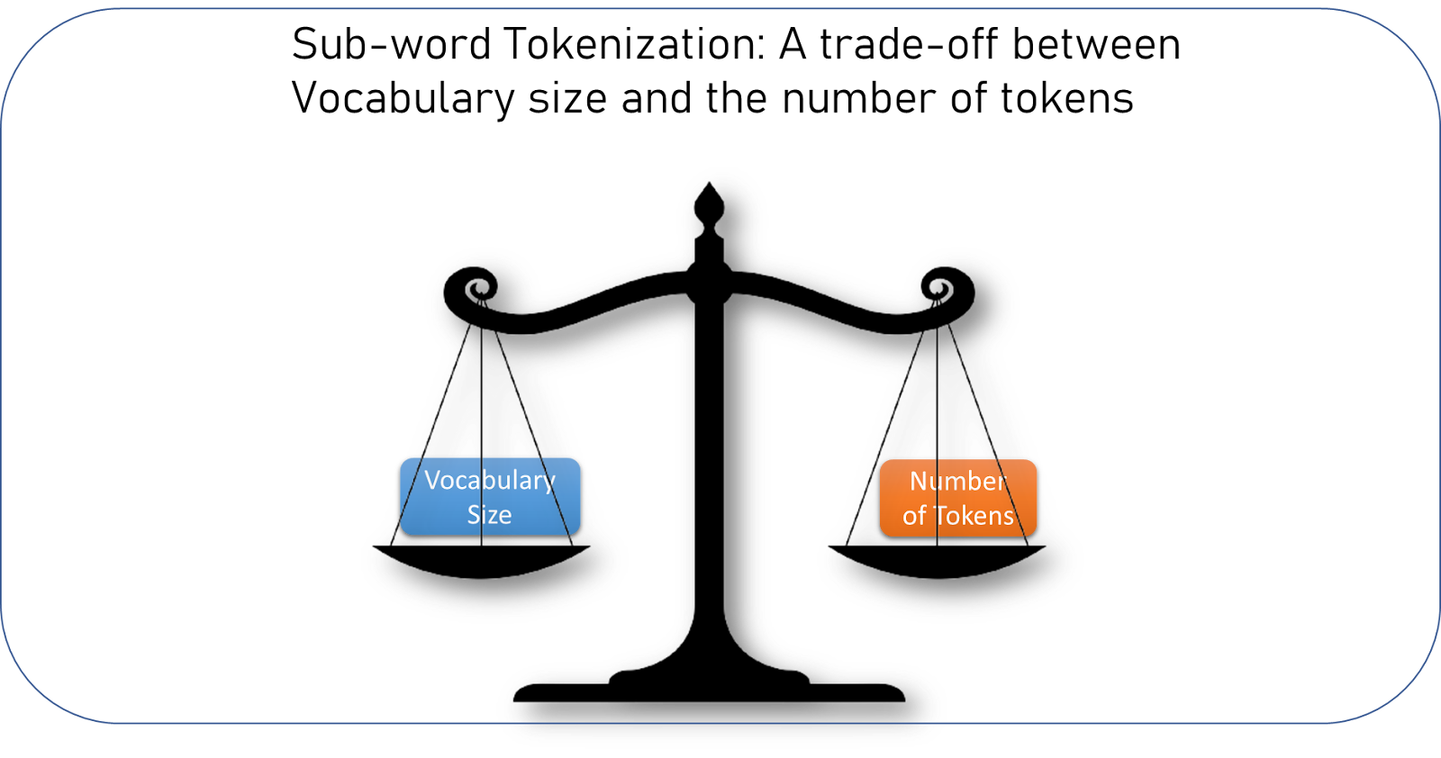
Figure: A trade-off between vocabulary size and no.of tokens (this could never be a consideration for smaller datasets). More importantly, for handling out-of-vocabulary context.
Embedding: Converting tokens to a vector of floating numbers
As you might already know embedding a token is nothing but converting/representing that token as a fixed-size 1D vector (768 is the dimension of that vector in "GPT-3 small" model). The embedding algorithms evolved over time. Here’s the timeline along with a brief explanation.
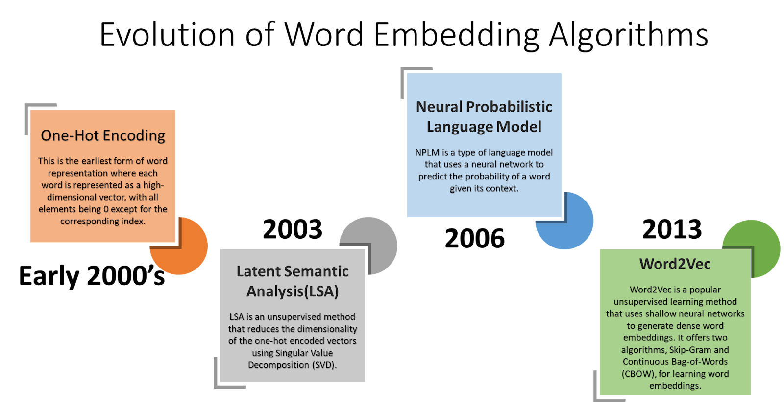
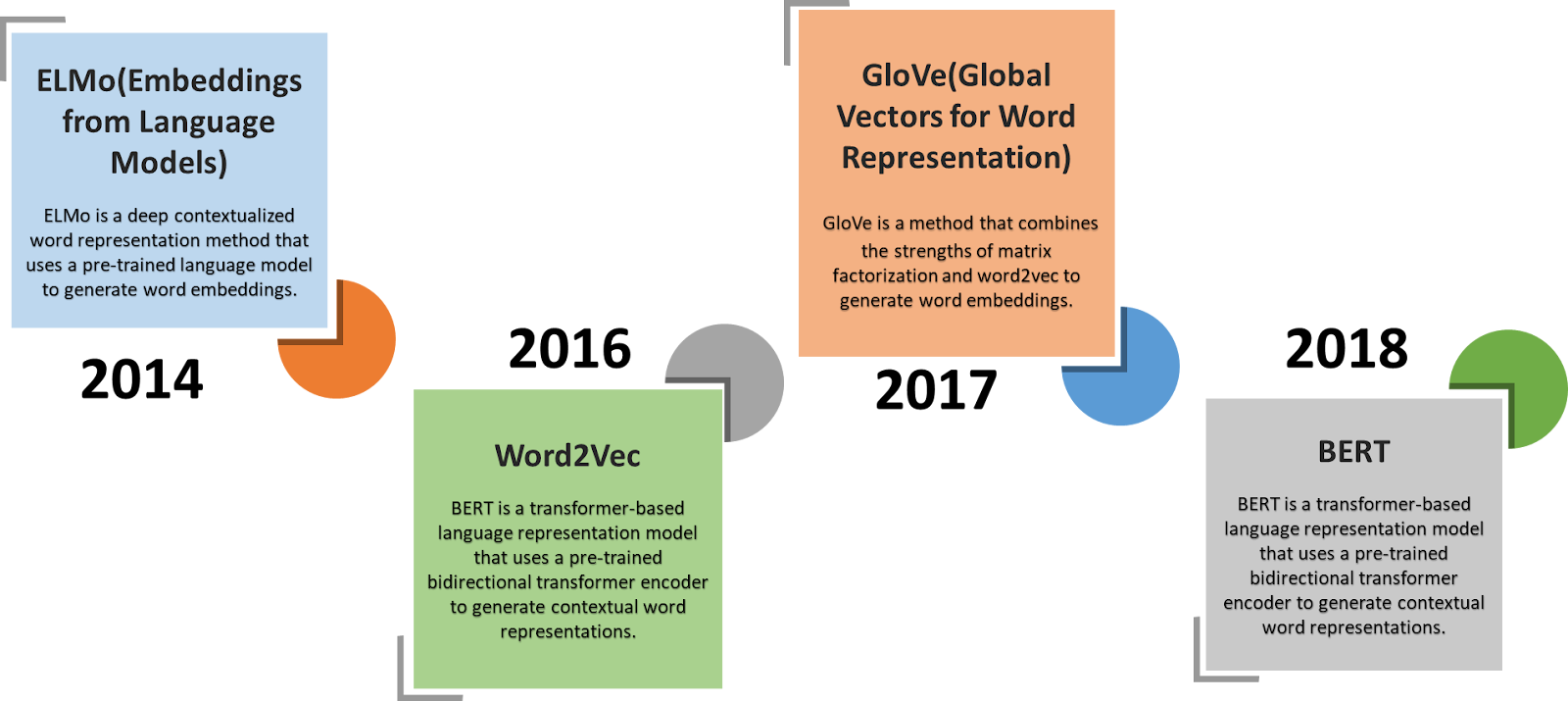
But OpenAI GPT-3 did not use any of these pre-trained vectors for their tokens. Instead, OpenAI GPT uses the Transformer-based language model architecture and trains its word embeddings during the model training process (in other words from scratch). It does not use ELMo (Embeddings from Language Models) which is a deep contextualized word representation method.
Summary So far
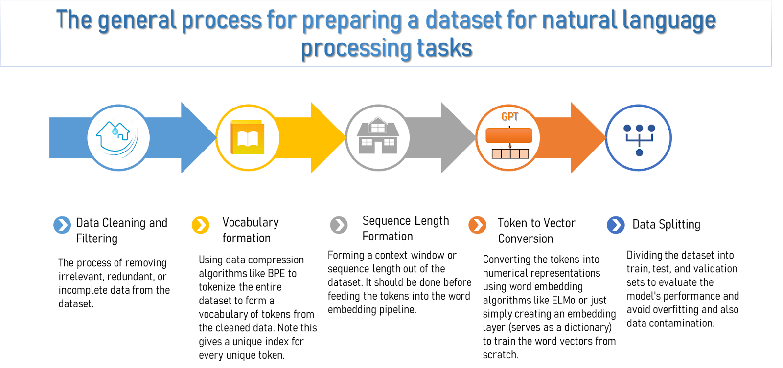
Figure: The general process for processing a dataset for natural language processing tasks
That’s enough of dealing with the complexity of dataset information. Also, I think so far I’ve put in a lot of information for you to gulp in. My apologies, I suggest you take a break and just ponder on what you’ve learned so far. If you’re done, time to look at another interesting part: GPT-3’s Model Architecture.
Model’s Architecture
Prerequisites before skimming through this section:
- Better Understanding of how Transformers work
- How decoders in Transformers work
- In transformers, the difference between self-attention, attention, and cross-attention
- How a Masked Multi-Head Self-attention Layer works

Believe me or not the above picture you’re looking at is exactly what happens but at a great scale i.e., the vectors in the above are quite bigger in the actual GPT-3 model. Indeed, the same vectors with the same size come out of GPT-3 model as shown in the picture. And this flow of vectors continues and that number is 300 billion!! There is another important point you have to remember. The above example (“GPT is Incredibly Powerful Model” (let’s say the target is “Model”)) constitutes 4 more examples for the model to train on. Here’s an illustration of what I mean.
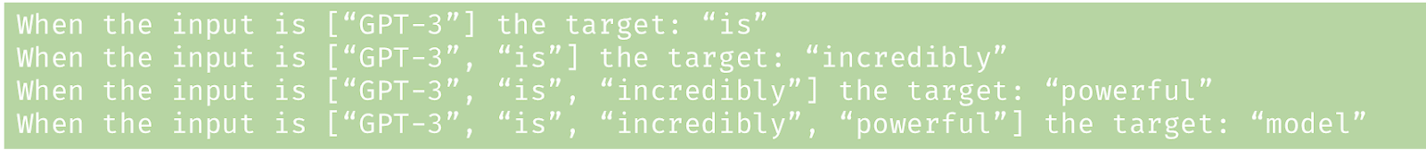
Figure: Every sequence (let’s say of length n) will constitute n examples within. Here I placed words for better understanding but in code, those words are mapped to their corresponding indices in the vocabulary.
And this happens for every sequence block we have. That is why the transformer’s decoder is known as an autoregressive model.
Ok, So here’s the OpenAI statement about GPT-3’s model architecture:
“We use the same model and architecture as GPT-2 including the modified initialization, pre-normalization, and reversible tokenization described therein, with the exception that we use alternating dense and locally banded sparse attention patterns in the layers of the transformer, similar to the Sparse Transformer”
And here’s their assertion on GPT-2’s model architecture:
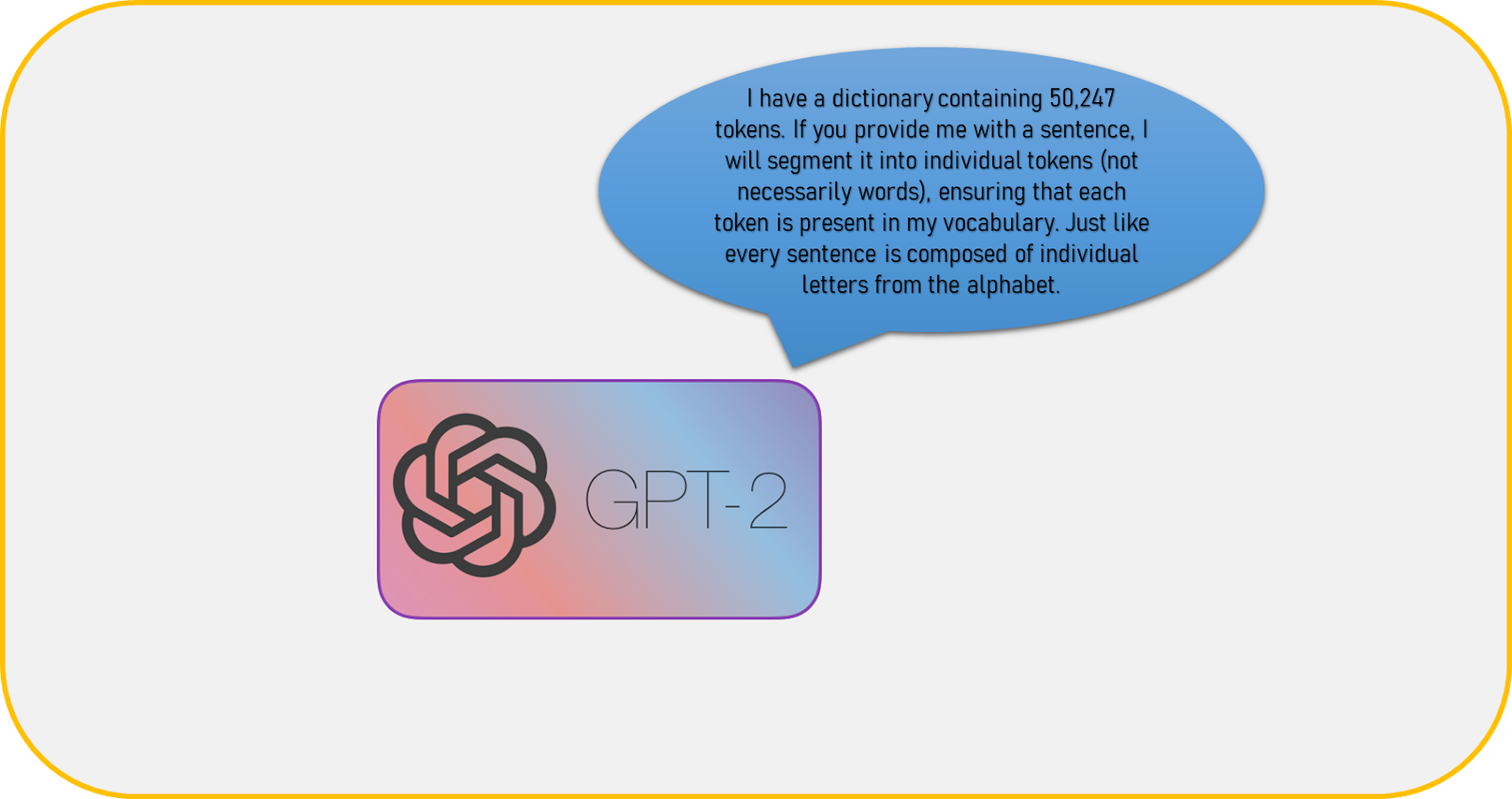
“Our language model is based on a Transformer architecture similar to OpenAI GPT with modifications such as input layer normalization, an added final layer normalization, and modified weight initialization. The vocabulary has been expanded to 50,257 and the context size increased to 1024 tokens with a larger batch size of 512. The residual layers have been scaled at initialization to improve performance.”
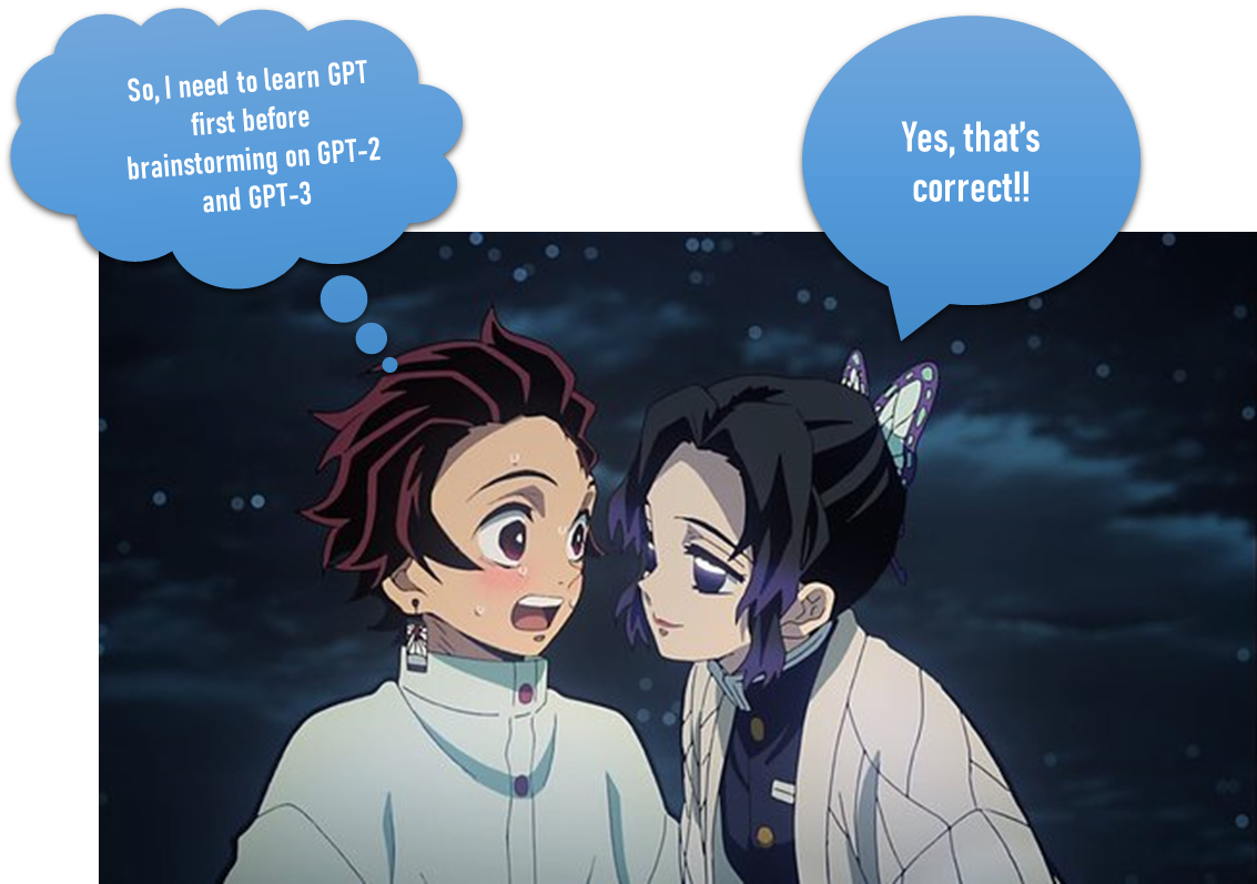
Here’s what I hope you’re thinking right now
Mathematical Intuition of Neural Networks
At a broader mathematical level, the work neural networks do is nothing but take in matrices, and manipulate them by multiplying or adding them to another matrix resulting in another matrix.
OpenAI GPT’s Working through Illustrations
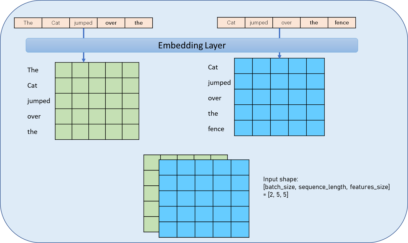
Figure: The above figure shows how “tokens” (I have put words for understanding purposes) are translated to vectors by the embedding layer and corresponding batch size of 2 with sample input shape.


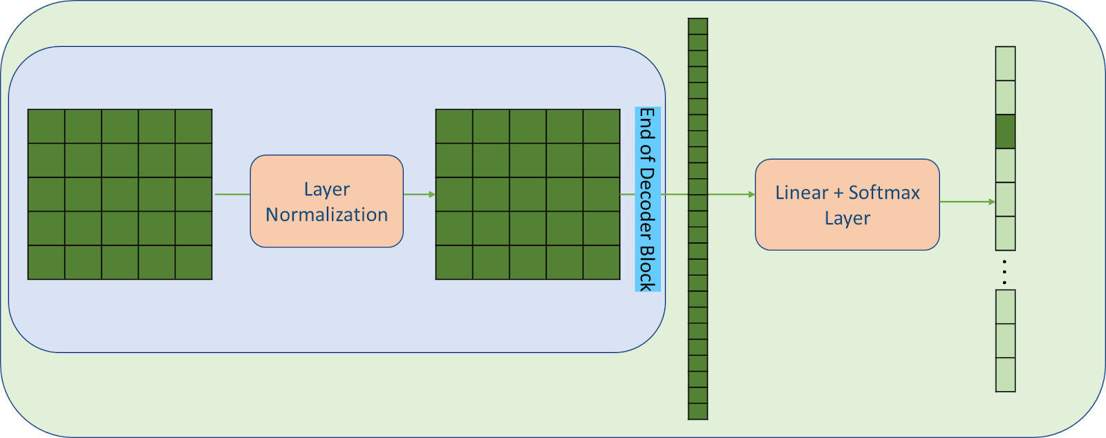
Finally, Here’s a broader picture of the architecture of OpenAI GPT
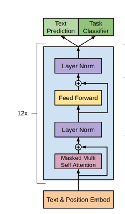
Figure: OpenAI GPT Model’s architecture
The above illustrations show how GPT processes a single sequence of tokens. The updated versions i.e., GPT-2, and GPT-3 are no different from this GPT except there are some differences in layers placement, and included are some changes in the weight initialization and some more which you have seen in the earlier paragraphs. (Read those paragraphs again and they will make much more sense now)
Training Details of the Model
Training Details of the Model at a theoretical level (i.e., omitting the number of GPUs, how they are used for parallelization, hardware failures, etc…) encompass information about the following:
- Hyperparameters i.e., number of decoder layers used, sequence length or context size, number of multi-heads used in masked self-attention layer, etc…
- Learning rate
- Optimization scheme (Adam’s Optimization)
- Backpropagation algorithm used (Stochastic Gradient Descent)
- Loss function utilized (Cross-entropy)
- Batch Size and so on…
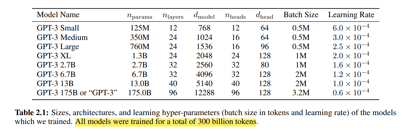
- n_params: This refers to the number of parameters in the model. In this case, it's 125 million. It’s just a count of the number of elements in weight and bias matrices of all layers in the model.
- n_layers: This refers to the number of decoder blocks GPT-3 models have. The number of layers in a model determines its depth, and deeper models tend to perform better on complex tasks.
- d_model: This refers to the size of the vector of each token. In the case of GPT-3 small each token is represented as a vector of size 768.
- n_heads: This refers to the number of heads in the multi-head attention mechanism used by the model. In this case, there are 12 heads. Multi-head attention allows a model to attend to multiple parts of an input sequence simultaneously, which can be useful for tasks like machine translation and summarization.
- d_head: This refers to the dimensionality of each head in the multi-head attention mechanism. In the case of GPT-3 small, it's 64. In other words, it is the vector size of each token that comes out of the head of each multi-head attention layer. The dimensionality of each head determines the capacity of the attention mechanism, and larger dimensions can help a model better capture the relationships between input and output.
- Batch Size: This refers to the number of examples used in each training iteration. In this case, it's 0.5 million. The batch size determines the memory and computational requirements of training, and larger batch sizes can speed up training but require more resources.
- Learning Rate: This refers to the step size used during gradient descent optimization. In this case, it's 6.0 x 10^-4. The learning rate determines how quickly the model updates its parameters during training, and too large a learning rate can cause the model to overshoot the optimal solution, while too small a learning rate can cause the model to converge too slowly.
So, finally, we’re done with the pre-trained model. What’s next? Well, it’s time to focus on meta-learning a new concept introduced by OpenAI starting from their GPT-2 model. And we’ll learn about this and more through interesting illustrations in my upcoming blog together.
That’s all I have to present to you! Not gonna lie, this is still an exhausting blog for you to go through. By far this is one the most computationally expensive (in time) blog I’ve ever written. Hope you learned something to explain to other people. Happy Learning!! And also hope I’ll get in touch with you in another blog post.