The Story of Large Language Models(LLMs): Learn How They are Built from the Ground Up

Introduction

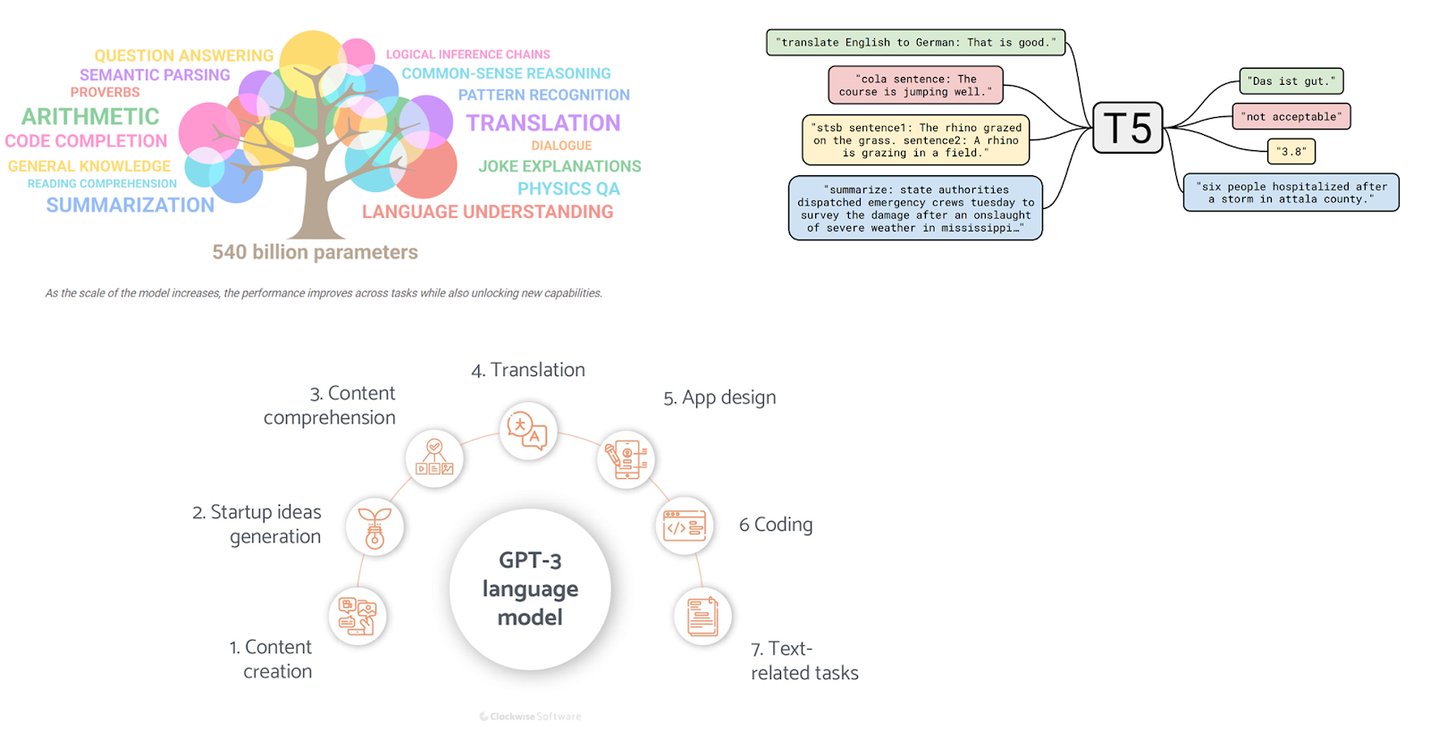
Large Language Models(LLMs) are a buzz these days. Models like GPT-3, PaLM, T5, BERT, and so on... have pushed state-of-the-art (SoTA) results in the NLP world to a new level. Even a complete novice person who doesn’t have any prior knowledge of the machine-learning world is able to experience an ocean of applications offered by these gigantic models. Especially, if it isn’t for OpenAI, unlike other AI organizations, which released all the models it developed in a way even a normal person can interact with and appreciate, making the world realize that something big is happening. The API playground it offered, and the websites it made to interact with its models (chatGPT for example) really should be appreciated since no other organizations have really come close to demonstrating their innovations to the normal public as OpenAI does. 

Coming straight to the point, this blog is so wordy and might be difficult to go through in one go so go through this if you’re in the right mood. This article is just a culmination of information on how Large Language Models are built from the ground up i.e., data they use to train on and the deep inner workings. And this is done by comparing various LLMs simultaneously. So, this blog will be useful if you are working on a team that builds LLMs or just a curious person since as I mentioned before this blog gathers information about various LLMs in one place with some simple explanations and illustrations.

Step 1: Getting and Pre-Processing the Data

This is where the problem begins. We need text to train our neural network model, correct? The more data, the better the model. Nowadays, it’s really easy to get an unprecedented amount of text from the internet thanks to the Common Crawl which does that operation and stores this text data in various formats. But one should be able to answer the following inferences if they want to feed this “raw text” directly to their neural network model:

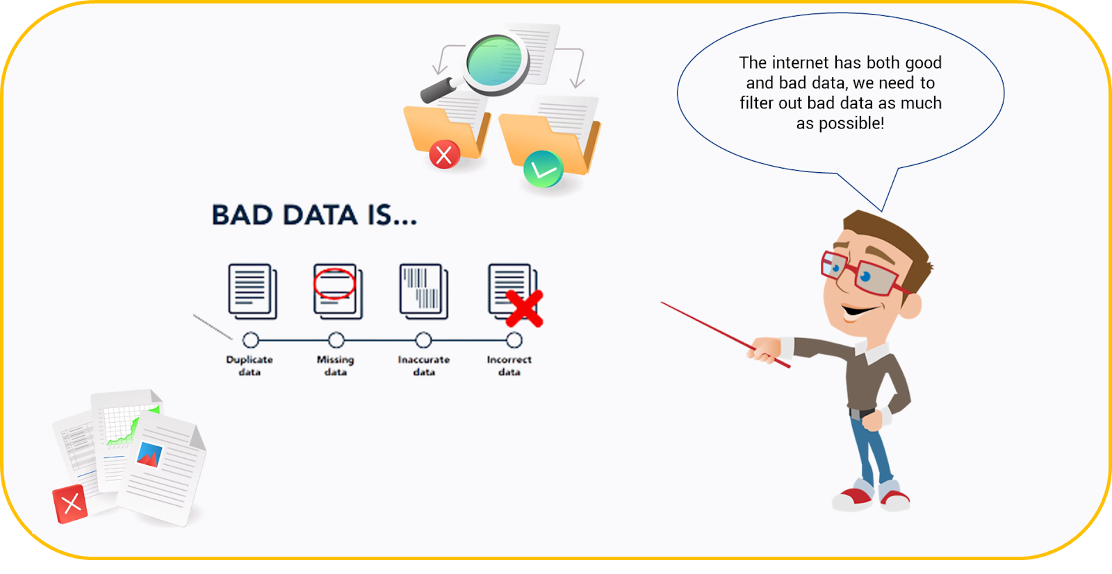
• The internet is a mess, and all the faults in documents, sentences, and, words across the world wide web like meaningless, duplicate documents, untruthful and low-quality sentences, misspelled words, and so much more which we sometimes cannot even guess, and even cannot list them down one by one. 
• But we just know one thing, i.e., we know what good data looks like rather than thinking of possibilities of how bad data looks. So, how can we get this good text data i.e., high-quality documents with good use of vocabulary and well-organized sentences and words from the internet which encompasses bad data as well?
• Typical preprocessing NLP techniques like removing stop words, converting upper to lower cases, and other stuff don’t make sense anymore since we want our LLMs to generate human-like text so every little detail has to be preserved. So, How do we preprocess or filter or clean the datasets we collect?

Let’s see how big AI organizations have answered the above questions through their research: 

OpenAI’s GPT Family

As I have mentioned earlier, OpenAI’s GPT models are well-known, especially GPT-3 which has brought chatGPT among us. It is right to say that they started small and raised the levels thereafter. You’ll see what I mean in a moment.

For training the GPT model they have collected the BookCorpus Dataset which has thousand of unpublished books from various genres like Adventure, Romance, etc… As you might have guessed, GPT-1 isn't trained on the internet but we can say to an extent that they collected a high-quality dataset since books as we know contain good text compared to the whole internet garbage. So, no worries about preprocessing steps here (standardizing some punctuation and whitespace is more than enough). Also at that moment OpenAI really wanted to experiment with model architecture more than pondering on the dataset. 

Time for GPT-2 to level up the amount of text data it gets to train on. So, they realized as we discussed earlier a large and diverse dataset like Commoncrawl (which has nearly unlimited text) has significant data quality issues and the content is mostly unintelligible i.e., bad data. But if we think about the key to collecting good data then we have one reliable source i.e., human intelligence since as humans we only like to read webpages with good text data. So, they’ve done the following in hopes of getting good data i.e., they scrapped all outbound links (a link from Reddit to an external website), about 45 million links 😲 in Reddit, which received at least 3 karma (users score, totaling their amount of upvotes against their downvotes) resulting in a new dataset which they named as WebText. Unfortunately, WebText hasn’t been released publicly but the one that is closest to is OpenWebText

Pre-processing Phase

During preprocessing phase, they removed all Wikipedia documents and performed de-duplication (removing duplicate documents) and some heuristic-based cleaning (See the list below)

A Note on Heuristic-based Cleaning

Heuristic-based cleaning involves using rules or algorithms to clean or filter data in a dataset based on experience or common sense. Some possible heuristic-based cleaning approaches that may be used to clean a text dataset like WebText include:

1. Remove documents or web pages with a low word count or content quality.
2. Filtering out pages that are not in English.
3. Eliminating pages with broken or missing links.
4. Removing pages with a high proportion of advertising or spam content.
5. Filtering out pages that are duplicates or near-duplicates.
6. Removing pages with irrelevant or uninformative content, such as placeholder pages or login pages.
7. Removing HTML tags or other formatting elements from the text etc… (kind of depends on the dataset collected)

As time progressed, OpenAI realized their model architecture is successful in comprehending text, but also the time has come to make their model look at the entire internet (Common Crawl Dataset) since the model has to know everything in order to be reliable and practical for everyone but the long unanswered question still persists “how do we deal with the mess in the internet?”. As it turns out the answer is just to keep the bar of good text data as high as possible than the bad text data so that the model is susceptible to generating good text rather than bad text. That’s exactly what the organization has done while dealing with the CommonCrawl dataset it has collected to train GPT-3:

Pre-Processing Phase

1. Filtered CommonCrawl: An automatic filtering method was developed to improve Common Crawl's quality. A logistic regression classifier was trained on high-quality documents and used to prioritize and sample Common Crawl documents based on predicted quality scores.
2. Fuzzy deduplication: To prevent overfitting, documents with high overlap were removed using Spark's MinHashLSH implementation, and WebText was removed from Common Crawl. This decreased dataset size by an average of 10%.
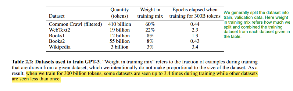
3. Added known high-quality references corpora like the expanded version of WebText, two internet-based books corpora (Books1 and Books2), and English-Language Wikipedia to the training mix to augment CommonCrawl and increase its diversity.

Google’s 540B PaLM Model

Unlike OpenAI, Google has a lot of experience and expertise in collecting good data since its primary search business focuses on delivering high-quality and trustworthy content to its users. So dataset collected to train the PaLM model has high-quality filtered web pages, Wikipedia, news articles, source code, and social media conversations. One perk is the same datasets are used to train both Google’s conversational LaMDA model and the 1.2T parameter GLaM model as well.

Pre-processing Steps

• A quality score was assigned to webpages using a classifier trained on known high-quality webpage collections. Webpages were sampled proportional to their score, prioritizing higher quality pages but not eliminating lower quality pages entirely.
• They have filtered the files by the license included in the repository excluding copyleft licenses which many AI organizations don’t do. 
• Removed duplicates based on Levenshtein distance between the files.
• Data contamination is employed after dividing the data into training and validation data since you want your model to predict data that is different from training data for true validation loss.

What do I do with this information?

Unless you’re working as a research engineer in one of the big Tech companies this information isn’t going to get you so far in building your own neural network model since dealing with this amount of data and infrastructure to train the model with isn’t something you can have right away. But the following points can be your takeaways:

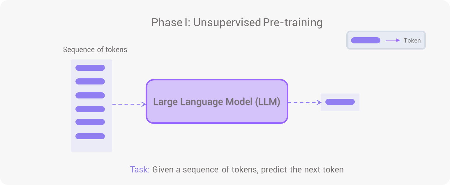
1. The task of Language modeling is to predict the next token given a sequence of tokens and through this process of prediction, we want our model to generate human-like text. Hence typical NLP pre-processing techniques like removing punctuations, lowercasing, stemming, removing stop words, etc.. shouldn’t be performed.
2. Instead, apply Heuristic-based cleaning (see the list mentioned above) based on the dataset you’ve collected.
3. Expertise in Descriptive Statistics is really crucial in these cases since extensive data analysis is damn important than anything. Helps in quantifying good data, gives sufficient evidence for Data Contamination (overlap between training and validation data), also to what extent the model is memorizing the data so on…
4. Training a classifier is really a good idea to clean and filter out datasets i.e., developing AI models in this area should be of utmost importance. 

Step 2: Tokenization and Embedding

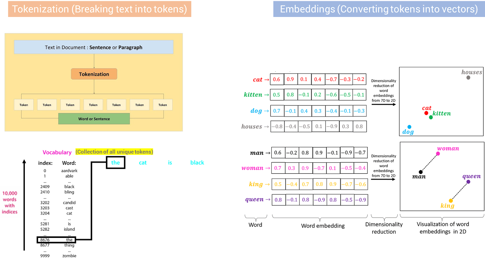
Let’s assume we’ve done everything that we can do to the data i.e., maximizing the likelihood of the presence of high-quality text data over poor quality. It’s time for tokenization, which simply means breaking down the text into tokens (note that the token may be a character, word, or subword). Why are we doing this? Well, that’s how language modeling task works, remember? (predicting the next token given a sequence of tokens). Basically, you’ll get two things when you perform tokenization:

1. Vocabulary which is a set of all unique tokens 
2. The Total Number of Tokens for your dataset

Before tokenization, we again have to answer a series of questions:

• The model can learn that a sentence has ended when there is a full stop(“.”) and follow-up space (in most cases) for a word, right? But how can we teach it a document has ended?
• This is where special tokens come into the picture. Various LLMs use different types of special tokens which commonly differ from each other. 
• When should we add special tokens before tokenization or after tokenization, if after tokenization and forming batches of sequences is it to start or end, or both, or some random places in a sequence? Should this be done by some rules?
• Also, how can we teach our model when should it end up generating text? For example, if I want my model to answer a question then it should end right after it generates a sufficient answer. Note that you don’t have to bother about this during the pre-training phase (language modeling) phase of the model, you can teach your model later as to when should it end its response. But for the zero-shot setting, we need to think about it. 
• As vocabulary size increases, the total number of tokens decreases and vice versa. Is there any optimal rule stating which one to prioritize more vocabulary size or the number of tokens? (Turns out you need to give priority to the vocabulary size)

Let’s explore how big LLMs have answered through their work.

OpenAI’s GPT Family

OpenAI's first version of GPT used Byte-Pair Encoding (BPE) to create its vocabulary. Basically, it does 40,000 merges on the training corpus (this would make sense if you know a little about the BPE algorithm). Sadly, they didn’t mention either the vocabulary size or the total number of tokens and no details of special tokens. But the BPE algorithm is the one you can take note of.

Before talking about tokenization, GPT-2 addresses the problem of either choosing a Byte-level Language model or a word-level language model. Typically, words are fed as (converted to) embedding vectors (referred to as encoding) while loading them into neural network models. This indeed is a word-level language model. Whereas in byte-level you have bytes (recall a byte consists of 8 bits (0s or 1s)) instead of words. So the model is predicting the next byte given a sequence of bytes. The question that should strike you immediately is “Why should we even consider going with bytes when we can deal with words?”. Both language models have their own pros and cons but the answer to the above question can be answered nicely with one single difference table.

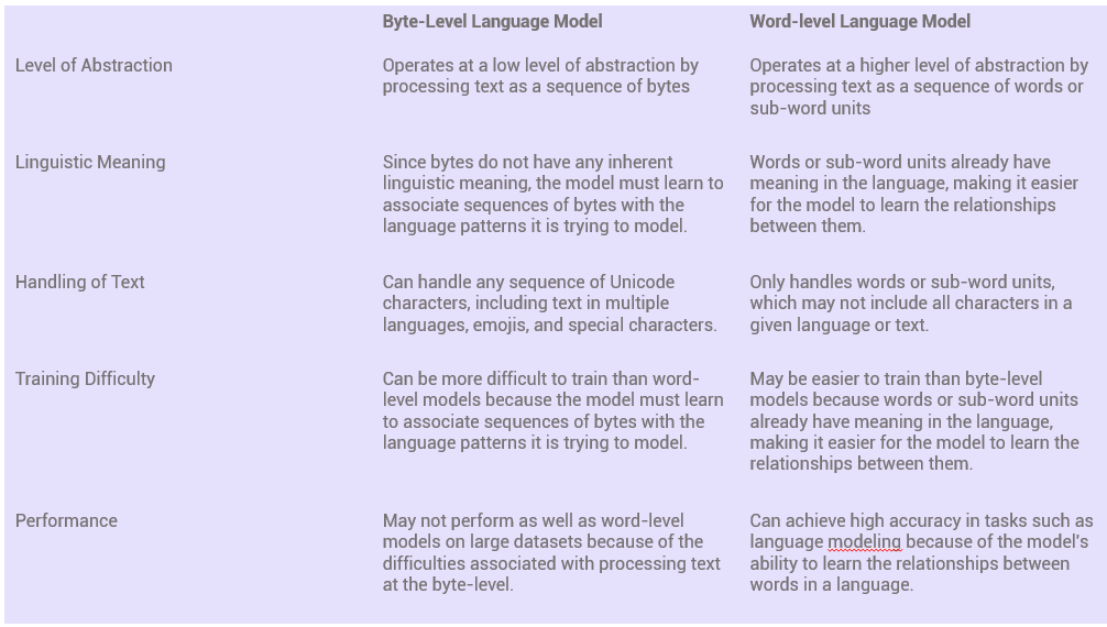
• Vocabulary Size and Handling Out-of-Vocabulary (OOV) tokens: In simple words, with word-level tokenization, the size of vocabulary size will be larger, and dependent on the dataset, and at the same time any unknown word (when we use a test dataset to test our model on various tasks) which isn’t in the vocabulary can’t be dealt with. On the other hand, byte-level tokenization has a fixed-size vocabulary of the size of 256 and can handle any sequence of Unicode characters, including text in multiple languages, emojis, and special characters but falls behind in performance when handling large-scale datasets.

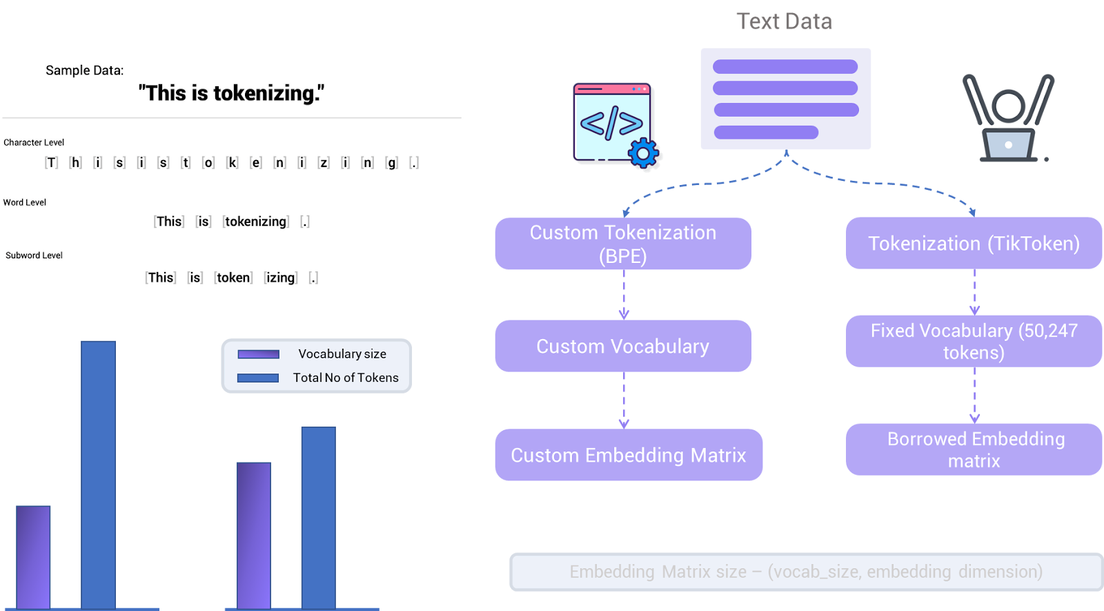
Which one did GPT-2 choose then? It has chosen sub-word level tokenization using a Byte-level Encoding (BPE) algorithm which offers the best of both byte-level and word-level worlds. The BPE algorithm works by iteratively merging the most frequent pairs of contiguous bytes in the corpus until a predefined vocabulary size is reached. Hence after tokenizing with this particular tokenization algorithm (under some specific rules) the vocabulary size of GPT-2 is 50,247 tokens. Indeed GPT-2 now open-sourced this vocab size and the corresponding tokenizer so that you can use it for tokenizing your dataset (Note that the vocab size is fixed i.e., 50,247) and they named it as tiktoken

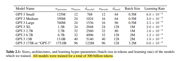
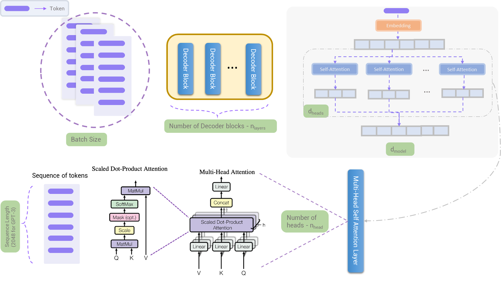
GPT-3 uses the subword-tokenizer with a fixed vocabulary size of 50,247 tokens developed during GPT-2 (on WebText) over its gigantic dataset corpus resulting in 300 billion tokens for the model to train on. And the next thing i.e., after tokenizing is forming a sequence array of 2048 tokens (context size or block size) in length, if a document is smaller than 2048 then it is merged with another document separated by a special <|endoftext|> token. 

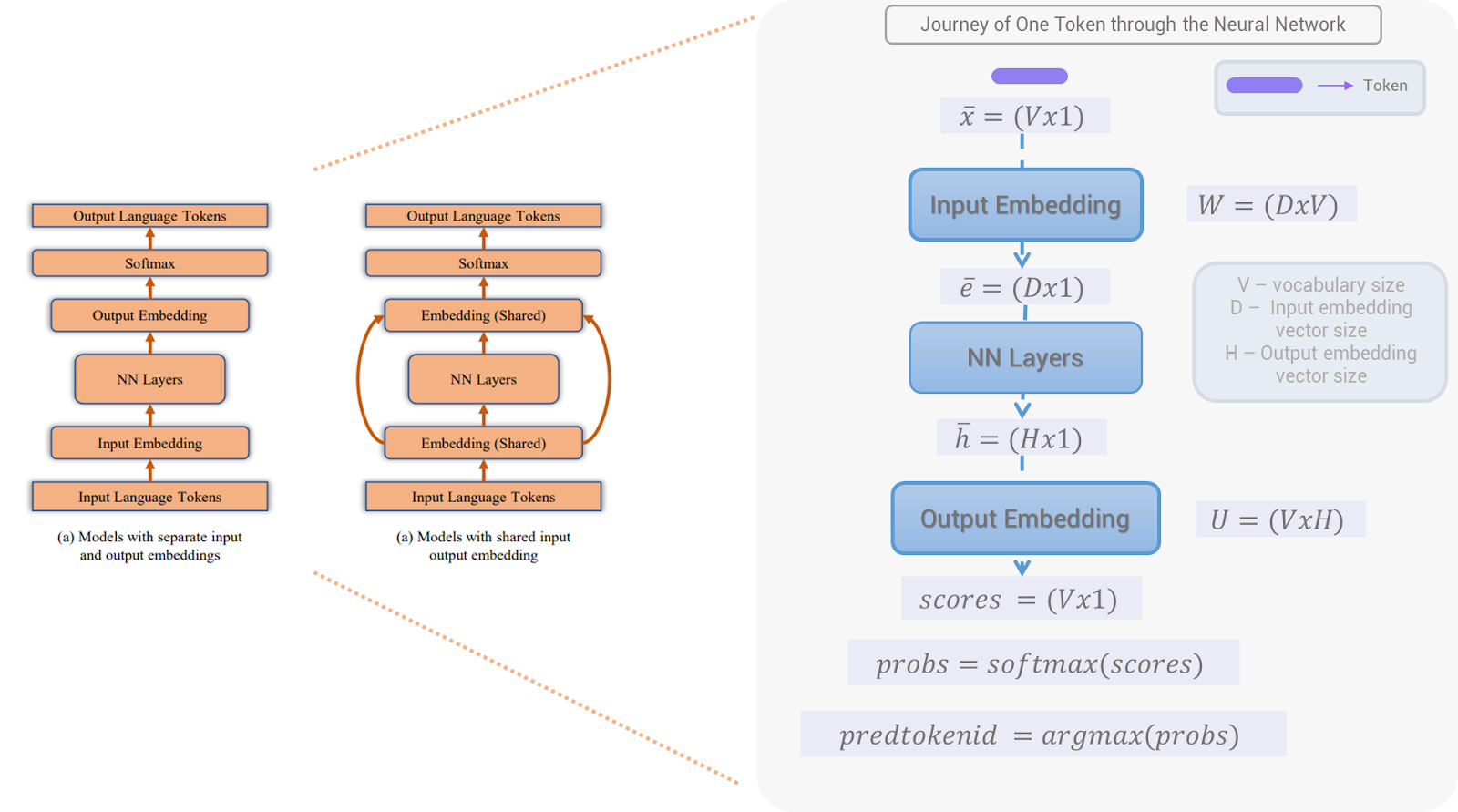
GPTs didn’t use any pre-trained embedding matrices instead they initialized a random embedding layer and tuned it while training. This makes sense because they built their own vocabulary. 

Google’s 540B PaLM Model

 After a thorough data analysis of quality data and data contamination between training and evaluation data, it’s time for tokenization. They used SentencePiece Tokenizer applied only on training data (which internally uses the BPE algorithm) which has a fixed vocabulary with 256k unique tokens (which support a large number of languages) creating 780 billion tokens in total. Further, these tokens are split into sequences each of length 2048 (same as GPT-3). Different input samples (documents) if present in the same sequence are differentiated using the <eod> token.

• Thereafter, one-hot encoded tokens are converted into numerical dense vectors (embeddings) by an input embedding matrix whose size is given by (vocab_size, embedding_dimension). After going through the network and output embedding matrix we get the output of the network, a vector of size (vocab_size, 1), which is compared against the vocabulary to determine the next output word. 

• RoPE (Rotary Position Embedding) Embeddings instead of traditional positional embeddings for performance reasons.

What are the things that I can experiment on?

• One important thing to note here is if you’re working on your own dataset, then instead of developing a tokenizer of your own you can use these open-sourced tokenizers with fixed vocabulary size and load their embedding weights into your model.
• Hence one should consider experimentation with tiktoken and SentencePeice tokenizers for their models. 

Step 3: Model’s Architecture

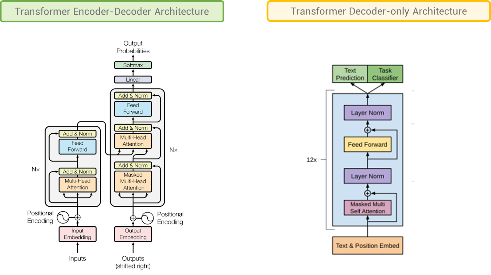
Before diving into the details, it is really worthier to know that this is the area where anyone even an ordinary person can bring in innovations. For instance, AlexNet, created by Alex Krizhevsky is the first CNN model architecture to win the ImageNet competition. Anyways, coming back to the topic, a breakthrough happened in 2017 in the NLP world which no one saw coming. It’s a research paper titled “Attention is all you need” published by Google introducing a new architecture that will change the way neural networks understand text i.e., Transformers to the world. Soon after its introduction, the world of RNNs, LSTMs, and GRUs rendered useless, and in just a few years every model that is developed borrowed the Transformer's architecture idea in some way or the other. For example, the GPT family uses Transformers decoder-only architecture, BERT uses Transformers encoder, and the T5 framework uses both encoder and decoder to frame themselves as Large Language Models (LLMs). The ability to understand long sequences and their parallelization processing capability kept transformers on the throne which previous RNN-based architectures failed to achieve. 

As you might have not guessed, it is important to understand how Transformers work before drenching yourself with Large Language Models (LLMs) architectural details. I recommend you go through the illustrated guide to transformers by jay alammar's blog to get a grip on it.

OpenAI’s GPT Family

As I mentioned earlier, the GPT family uses decoder-only Transformers. GPT-1 model has 12 decoder blocks. A decoder block further comprises two things: a self-attention layer and a feed-forward neural network (MLP). The following list summarizes the details:

• Decoder-only Transformer with 12 decoder blocks, masked self-attention heads (present tokens do not see the values of the future tokens) with 12 attention heads, and the output size (coming out of decoder block) of each token is 768 (embedding size). For FFNN, the number of neurons in the hidden layers is 3072 (768*4 always) each. 
• Gaussian Error Linear Unit (GELU) is used as an activation function and randomly initialized positions embedding matrix (elements are tuned while training) rather than the sinusoidal version proposed in the transformer.
• LayerNormalization is used, also weight initialization between the values (0, 0.2), residual connections, embedding, and dropout with a rate of 0.1 for regularization is employed.

 GPT-2, and GPT-3 have the same configuration but the details of how many decoder blocks are used, and other internal details change. Let’s read in their own words:

For GPT-2: “Our language model is based on a Transformer architecture similar to OpenAI GPT with modifications such as input layer normalization, an added final layer normalization, and modified weight initialization. The vocabulary has been expanded to 50,257 and the context size increased to 1024 tokens with a larger batch size of 512. The residual layers have been scaled at initialization to improve performance.”  Here’s the summary

• Same as GPT-1 with few modifications. Layer normalization was moved to the input of each self-attention block (pre-activation) and the additional layer norm was to the final self-attention block
• Scaled the weights of residual layers at initialization by a factor of 1/ √ N where N is the number of residual layers.
• The batch size is increased from 64 to 512 and each batch now has a sequence length of 1024 tokens instead of 512 tokens. 

For GPT-3:  “We use the same model and architecture as GPT-2   including the modified initialization, pre-normalization, and reversible tokenization (removes tokenization / pre-processing artifacts) described therein, with the exception that we use alternating dense and locally banded sparse attention patterns in the layers of the transformer, similar to the Sparse Transformer”

Before going any further, I think it is important to ponder the following questions:

• How do researchers decide upon the choice of hyperparameters to choose and the position of the layers for the model? 
• Like in the case of GPT, how many decoder blocks should we use, the choice of the number of attention heads, the head size (output vector size of each token) of each attention head, embedding dimensions for a token, the number of hidden layers in FFNN, the dimensionality of the hidden layer, which activation function to try and so much more to decide upon. 
• There is indeed no specific answer to these questions, rather than trying out empirically using computationally inexpensive datasets. With each little experiment, you can spell out some words from the observations you make. For example, increasing self-attention layers makes the tokens talk to each other more, alleviating the size of FFNN gives the tokens more time to think about what they have seen from self-attention layers, and so on…
•  Also, from time to time, there are research papers that get published spelling out the inferences from the experiments they conduct on the model’s hyperparameters providing a well-informed initialization further.
• The story doesn’t end there, if you know how transformers work, there are some handful of hyperparameters inside the self-attention layer as well. Also, we need to make a decision on the context size (sequence block size) and the number of batches to feed in at a time to the model. 

Google’s 540B PaLM Model

PaLM also used the same decoder-only Transformer with some modifications in an effort to speed up the training process parallel to performance. 

Modification 1#: SwiGLU activation instead of standard ReLU, GeLU, or Swish activations 

Modification 2#: Parallel Layers rather than standard serialized formulation i.e., 

y = x  + MLP(LayerNorm(x) + Attention(LayerNorm(x)) instead of 

y = x + MLP(LayerNorm(x + Attention(LayerNorm(x)))

Modification 3#: Multi-query Attention

The standard Transformer model uses k attention heads, each of which linearly projects the input vector into query, key, and value tensors of shape [k, h]. However, here the key/value projections are shared across all heads (which doesn’t happen in a standard transformer), while the query projection remains separate. Although this does not affect the model quality or training speed, it significantly reduces the cost of autoregressive decoding, as the key/value tensors can be shared between examples, making it more efficient on accelerator hardware.

Modification 4#: No Biases were used in any of the dense kernels (weight matrices) or layer norms since this increases training stability for large models.

• Kernel weights (i.e., everything but the embeddings and layer norm scales) are initialized with “fan-in variance scaling”, i.e., W 
• No dropout layers are used

Think and Experiment with Model 

• Training Large Language Models (LLMs) often requires making a sacrifice, i.e. excluding some good details or optimizing them for faster training.
• Nevertheless, the answer to the choice of hyperparameters is purely statistical, i.e., conduct an experiment on computationally inexpensive datasets, and if the results improve, find out what is causing this improvement by providing an inference, and repeat the process by stacking successful experiments on top of each other.

Step 4: Training Details 

We can wrap up the entire story of training through the following paragraph:

Large data is collected, cleaned, tokenized,  converted to sequences, and finally divided into batches of training data ready to get fed into the model. Instead of feeding the entire data or batches only a fixed group of batches goes into the model one by one saving the computer’s memory (RAM). Thus the model learns from the flow of batches it receives. An epoch is a loop indicating how many times you’re making the model see the entire data (2 epochs mean the model has seen the entire training data two times). A step in an epoch means since we have batches to feed, one batch that goes into the model input pipeline corresponds to one step. Therefore, the total number of batches is equal to the number of steps per epoch. 

That’s a typical theory about training everyone knows of, but there is another interesting way to train your model. Basically, feeding huge amounts of data (Common Crawl for example) more than once is a daunting task and it is computationally expensive. Instead, what LLMs researchers do is they shuffle their batches of training data and train their models by sampling the batches using either of the two options: sample a batch with replacement and sample a batch without replacement. The only hyperparameter that stays in this case and it is not epoch or step per epoch but is a new term named “iterations” meaning the number of random batches you sample from the pile of batches (6000 iterations means we are sampling 6000 random batches). Also, the training and validation losses are not calculated for the entire data during each iteration (computationally expensive again) rather they are computed after a specific number of iterations are exhausted referred to as evaluation interval and computed for only a fixed number of batches (for a sample in the entire population) which is referred to as evaluation iterations. 

Let’s go through the story of how different LLMs trained their models:

OpenAI’s GPT Family

GPT-1

Backward Pass Details

• Using stochastic gradient descent as the backward propagation algorithm, Adam's optimization scheme with a maximum learning rate of 2.5e-4 updates parameters for each batch, not for a group of batches.
• The learning rate was increased linearly from zero over the first 2000 updates and annealed to 0 using a cosine schedule. 

Overall Training Details

• Trained for 100 epochs (since Books corpus isn’t really a huge one to deal with) with a group of 64 batches (shuffled and randomly sampled) and each batch has a sequence length of 512 tokens.

GPT-3

Backward-pass Details

• “Adam with β1 = 0.9, β2 = 0.95, and  𝝐 = 10−8, we clip the global norm of the gradient at 1.0, and we use cosine decay for learning rate down to 10% of its value, over 260 billion tokens (after 260 billion tokens, training continues at 10% of the original learning rate). There is a linear LR warm-up over the first 375 million tokens. We also gradually increase the batch size linearly from a small value (32k tokens) to the full value over the first 4-12 billion training tokens, depending on the model size.”

Overall Training Details

• Data are sampled without replacement during training (until an epoch boundary is reached) to minimize overfitting. Each batch has a sequence of 2048 tokens.

Google’s 540B PaLM Model

Backward Pass Details

• “The model is trained with the standard language modeling loss function, which is the average log probability of all tokens without label smoothing. We additionally use an auxiliary loss of z loss = 10−4 · log2 Z to encourage the softmax normalizer log(Z) to be close to 0.”
• “We use an Adafactor learning rate of 10−2 for the first 10,000 steps, which is then decayed at a rate of 1/ √ k, where k is the step number. We train with a momentum of β1 = 0.9. The second-order moment interpolation value is computed as β2 = 1.0 − k −0.8, where k is the step number.”
• We use global norm gradient clipping with a value of 1.0 for all models. We use a dynamic weight decay of lr = 2.0 during training, where lr is the current learning rate. 

Overall Training Details

•  They trained all three models on exactly one epoch of the data (shuffled identically for all models) and choose the mixing proportions to avoid repeating data in any subcomponent.
• Batch size is increased during training with each data sample in a batch having 2048 sequence tokens. 

Key points to take away:

• Larger models use a larger batch size but require a smaller learning rate. 
• Our constant goal is to improve the training efficiency and give advantages to the model to learn to its maximum extent but sometimes we need to choose one at the cost of another. 

Conclusion for Effective Learning

In summary, we’ve journeyed from collecting and cleaning data and building the model to how the models are trained with that data. Though some of the details included may perplex you too much, nevertheless if you’re willing to start building an LLM on your own or help others to do the same then the time you spent on this article will definitely be worth it. As they say, experience speaks louder than words, you try to build a language model, GPT for example from scratch, then you’ll see the details discussed in this blog (i.e., the ways you can clean your data, various choices of tokenizers-embedding algorithms, the possibilities to build your customized model, and the effective way you can train and improve the efficiency of the model) reflect in your implementation for you to innovate better.