

- Published on
Advanced Visualized Guide for Learning Pytorch the right away
I remember using Keras as my deep learning library to build any neural network model. The reason why I picked it is quite predictable. Firstly, it was easy to wrap your mind around what was going on since the code itself explains a lot. Second, it abstracts or hides many details from you thus not reminding us of the need for customization. But as I progressed copying/pasting the code, I realized if you want to invent a model architecture with full customization (i.e., feeding it the data, training it, and testing it) yourself Keras doesn’t support you much in your way with the same coherence.
Thus any beginner would be presented with the two most popular options to support their ambition to build a new neural network on their own. Either go with TensorFlow or Pytorch. The choice is Pytorch for me. Why? Never tried Tensorflow because of this customization article. But it’s never bad to try something new, though!!
And so after building some neural network models in Pytorch, I realized the code is comprehensible just like Keras but now with customization!! (though didn’t realize this at my first shot). So, here’s what I am going to do to try to make you feel the same. Firstly, I am not going to trap you with a lot of words as I did with the previous paragraphs. Secondly, we’ll build a readable/comprehensible neural network model in Pytorch with best practices for a beginner through some visualizations. That’s it.
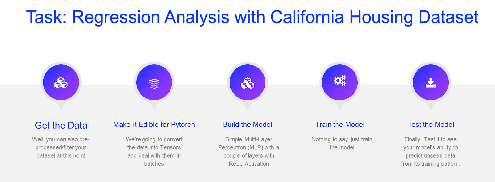
Table of Contents
- Getting the Data
- Make the Data edible for Pytorch Model Pipeline
- Build the Model
- Choice 1: Keras-Like Model
- Choice 2: Customized Model
- Train the Model
- Test the Model
- Visualization of the Model
- Proper Logic for saving the model while training
- Note on Overfitting
- Live Tracking the metrics
- Run Tensorboard in Google Colab
- Conclusion
So, In summary, you’re just going to look at five chunks of transparent code. Here's the entire code if you want to skip the article and just look at the code.
Getting the Data
# Import dataset
from sklearn.datasets import fetch_california_housing

# Extract the dataset
X, y = fetch_california_housing(return_X_y = True)


from sklearn.model_selection import train_test_split

# Split the dataset into train, test data
X_train, X_test, y_train, y_test = train_test_split(X, y, test_size=0.2, random_state=42)
# Split the train dataset further into train and validation data
X_train, X_val, y_train, y_val = train_test_split(X_train, y_train, test_size=0.2, random_state=42) # 60% train, 20% val, 20% test
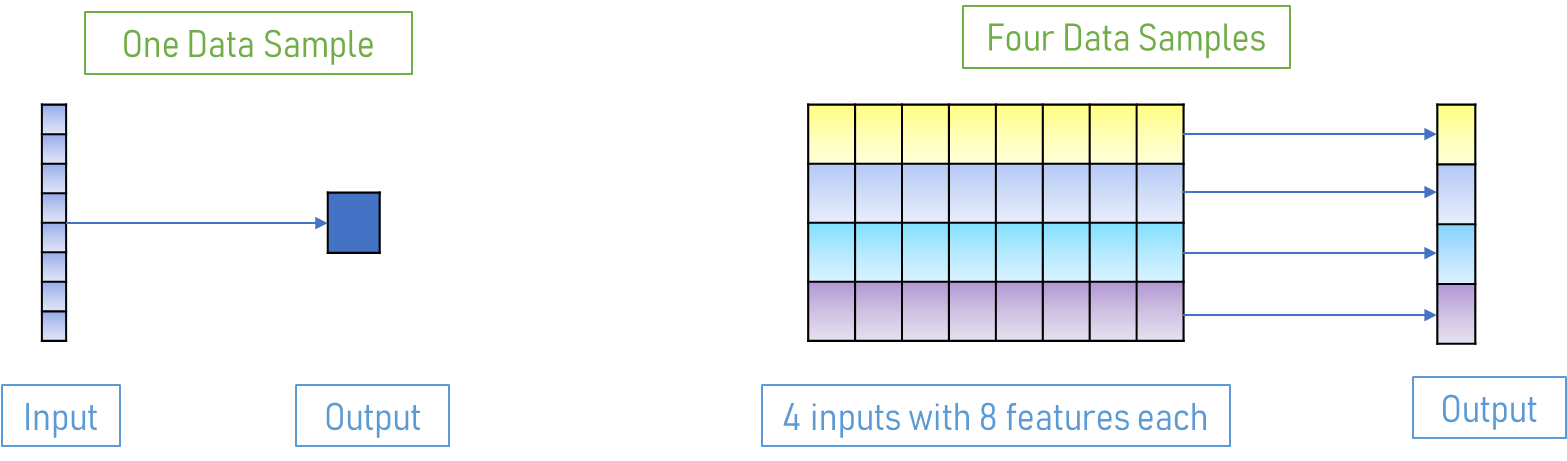
Nothing related to Pytorch here. Just loading and splitting the data is all we’re doing. By the way, a small note on the data, price i.e., the target is dependent on 8 independent values.
Make the Data edible for Pytorch Model Pipeline
# Make the data suitable to feedinto the pytorch model pipeline
import torch

# for input shape = (batch_size, 8) where batches = 20640/(batch_size), output shape = (batch_size, 1)
X_train = torch.tensor(X_train, dtype=torch.float32)
X_val = torch.tensor(X_val, dtype=torch.float32)
X_test = torch.tensor(X_test, dtype=torch.float32)
y_train = torch.tensor(y_train.reshape(-1, 1), dtype=torch.float32)
y_val = torch.tensor(y_val.reshape(-1, 1), dtype=torch.float32)
y_test = torch.tensor(y_test.reshape(-1, 1), dtype=torch.float32)


from torch.utils.data import TensorDataset, DataLoader

# Create a dataset class
train_ds = TensorDataset(X_train, y_train)
val_ds = TensorDataset(X_val, y_val)
test_ds = TensorDataset(X_test, y_test)

# Create data loaders for feeding the data in batches
batch_size = 64
# dataloader divides datasets into batches (one of the best practices)
train_dl = DataLoader(train_ds, batch_size, shuffle=True)
val_dl = DataLoader(val_ds, batch_size*2) # batch size for val, test is twice compared to train (quick evaluation)
test_dl = DataLoader(test_ds, batch_size*2)
Here are the Notes:
- Pytorch needs the data to be of type Tensors (not a list, NumPy array, or something) for automatic gradient accumulation/computation.
- In other words, Pytorch will do automatic differentiation (meaning you don’t have to write the steps for derivatives manually) with the help of tensors
- DataLoader divides our data into batches i.e., huge matrix into small slices of matrices to save memory. Because computers can’t read huge matrices (for huge datasets) loaded into them all at once.

Build the Model
Choice 1: Keras-Like Model
model = nn.Sequential(
    nn.Linear(8, 32),
    nn.ReLU(),
    nn.Linear(32, 2),
    nn.ReLU(),
    nn.Linear(2, 1)
)
Choice 2: Customized Model
import torch.nn as nn
import torch.nn.functional as F
from pytorch_model_summary import summary

class HousingModel(nn.Module):
    def __init__(self):
        super().__init__()
        self.linear1 = nn.Linear(8, 32) # kernel size
        self.linear2 = nn.Linear(32, 2)
        self.linear3 = nn.Linear(2, 1) # Output layer is a single neuron since we are predicting a single value

    def forward(self, xb):
        out = self.linear1(xb)
        out = F.relu(out)
        out = self.linear2(out)
        out = F.relu(out)
        out = self.linear3(out)
        return out

model = HousingModel()
Here are the Notes:
- In the first block i.e.,
def __init__(self)you just need to define the layers - In the second block i.e.,
def forward(self)you need to write the logic for the forward pass
Train the Model
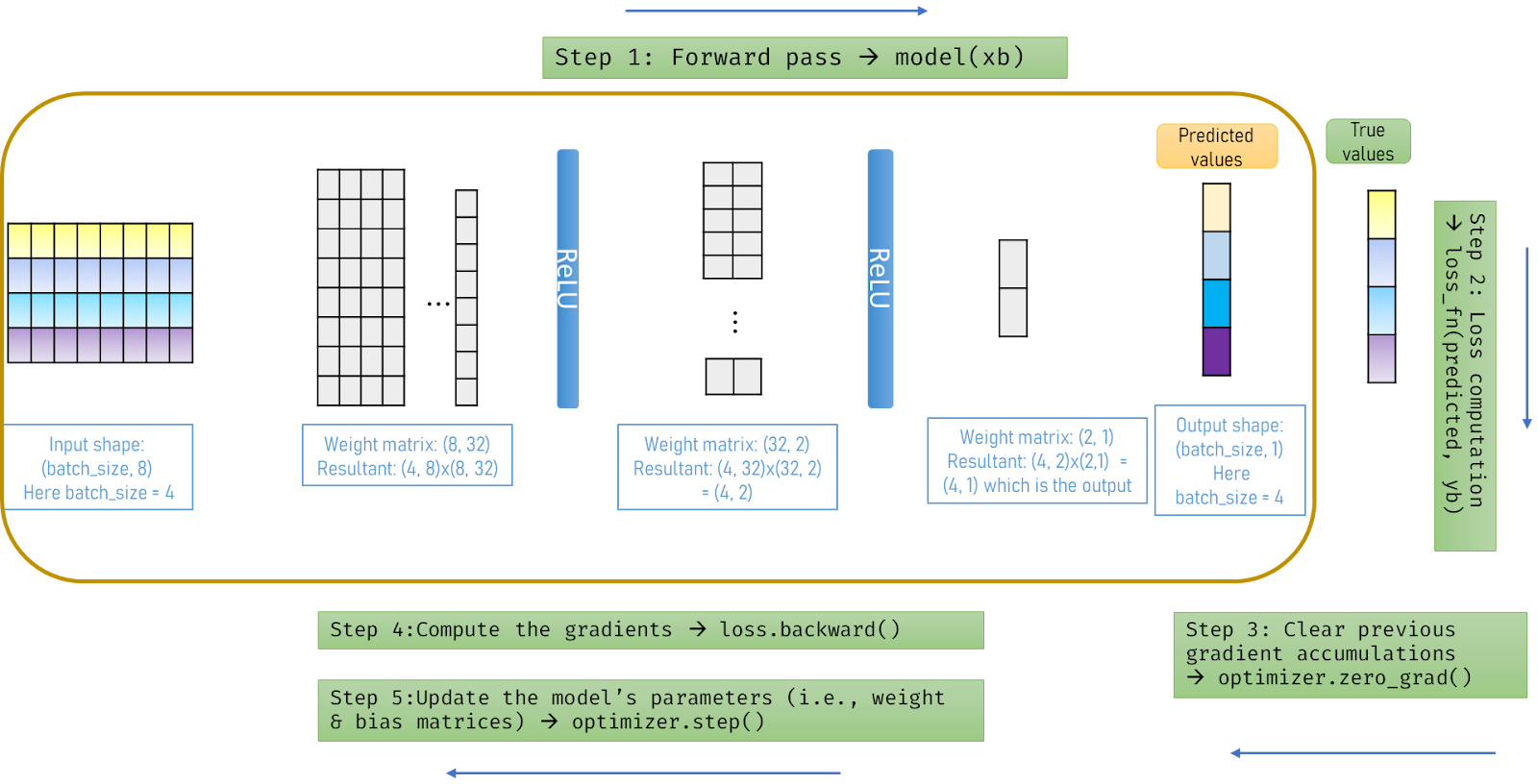
loss_fn = F.mse_loss # mean squared error loss
optimizer = torch.optim.SGD(model.parameters(), lr=1e-5)

for epoch in range(100):
    # lists that collect loss for all batches in one epoch
    train_losses, val_losses = [], []
    for xb, yb in train_dl:
        # outputs during forward pass
        pred = model(xb)
        # loss per batch between true and predicted values
        loss_per_batch = loss_fn(pred, yb)
        train_losses.append(loss_per_batch)
        # clear last batch size's accumulated gradients
        optimizer.zero_grad()
        # Perform gradient descent i.e., backward pass
        loss_per_batch.backward()
        # update model's parameters
        optimizer.step()
    # make sure no gradient accumulations happen since they occur during forward pass in pytorch
    with torch.no_grad():
        for xb, yb in val_dl:
            # forward pass (no gradient accumulations will during this forward pass)
            pred = model(xb)
            # validation loss
            val_loss_per_batch = loss_fn(pred, yb)
            val_losses.append(val_loss_per_batch)
    # average of all training batches in one epoch
    train_loss = torch.tensor(train_losses).mean()
    # average of all validation batches in one epoch
    val_loss = torch.tensor(val_losses).mean()
    # print the val loss and train loss for corresponding epoch
    print('Epoch [{}/{}], Loss: {:.4f}, Val Loss: {:.4f}'.format(epoch+1, epochs, train_loss, val_loss))
Here’s an illustration for the above code:
Well, this training process really got me the first time. Since in Keras, you don’t have to deal with these many lines for training your model. Just model.fit(X, y, validation_split=0.2, epochs=100) is enough. But the downsides of this approach are: (1) It abstracts a lot of logic about what’s really happening with the model which is really important to know (2) We are feeding the entire training data rather than in batches for our computer memory to store.
With PyTorch, you can overcome these disadvantages i.e., it makes you know more about what’s happening while training your model and offers a simple API (DataLoader function) to divide your data into batches. In other words, it offers comprehensible customization.
Here’s the Tensorflow code if you want to divide the training dataset into batches and then train the model
# Load the training data in batches of 16
train_dataset = tf.data.Dataset.from_tensor_slices((X_train, y_train)).batch(16)
# Train the model
model.fit(train_dataset, epochs=100)
But as I mentioned it just hides too many details (i.e., how validation logic is happening, how losses are calculated per epoch combining batches etc…) from you which isn’t good practice since you need to know this logic, especially about how you train your model.
Test the Model
# make sure no gradient accumulations happen during forward pass
with torch.no_grad():
    # list to collect losses across batches for one epoch
    test_losses = []
    for xb, yb in test_dl:
        # forward pass with no gradient accumulations
        pred = model(xb)
        # loss computation per batch
        loss_per_batch = loss_fn(pred, yb)
        test_losses.append(loss_per_batch)
    # print the overall loss
    print('Test Loss: {:.4f}'.format(torch.tensor(test_losses).mean()))
Here the logic is no different from the validation logic written while we’re training our model. As you know, the 7 lines of code here are translated to just 1 line of code in Keras i.e., model.evaluate(X_test, y_test, batch_size=128) but as mentioned earlier it just hides a lot of good details from you. Note that there is no accuracy metric for regression problems since that doesn’t make sense.
We’re done but hold on!! You may recall that I’ve mentioned “best practices” for PyTorch in my blog title. Are the above lines of code manifest them? The answer is absolutely no. Let’s see the extra lines of code we need to include for building and training our neural network model that most research practitioners use rather than writing the above theoretical code.
Visualization of the Model
As the model starts getting bigger, that is, as more layers and complex logic for forward pass evolves it gets too difficult to wrap your mind around what’s going on with your model. So, visualizing your model in these kinds of situations is damn important. For this, we’re about to do three things:
- Use Tensorboard to visualize our model as a graph
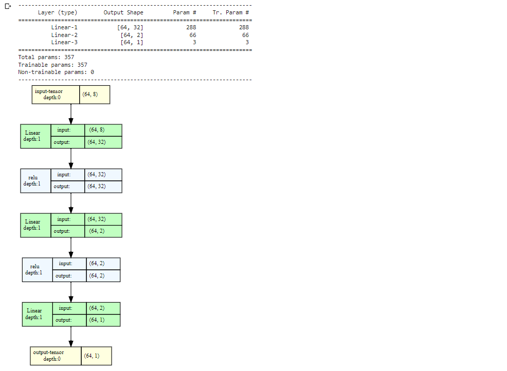
- Use the
pytoch_model_summarypackage for viewing the output shape at each layer, knowing the number of parameters as well - Use
torchviewto draw a simple graph with some colors
Here’s the code you need to include in the 3rd chunk i.e., Build the Model to visualize your model:
from torchview import draw_graph
from torch.utils.tensorboard import SummaryWriter
from pytorch_model_summary import summary

...
# Set up the tensorboard writer
writer = SummaryWriter()

def view_model(model, input_size, batch_size=-1):
    # *input_size is used to unpack the tuple i.e., (8,) to (8)
    inputs = torch.randn(batch_size, *input_size)
    writer.add_graph(model, inputs)
    print(summary(model, torch.zeros((batch_size, *input_size)), show_input=False))
    model_graph = draw_graph(model, input_size=(batch_size, *input_size))
    return model_graph.visual_graph

view_model(model, (8, ), batch_size)
Proper Logic for saving the model while training
We need three things to happen while training is happening at the same time:
- The model should be saved for every epoch so that if our training gets halted due to some reason, rather than training again from scratch, we can resume from the last epoch’s info.
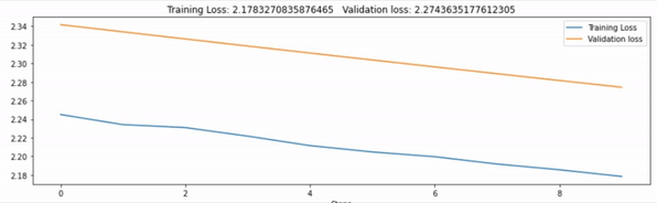
- Also, the model with the best validation loss should be saved, since if our model overfits (see illustration below), we don’t lose our model with the best validation loss. This is often referred to as checkpointing the model.
- Always save the final model in case, because it sometimes is the best model or when the model starts to overfit it isn’t.
Note on Overfitting
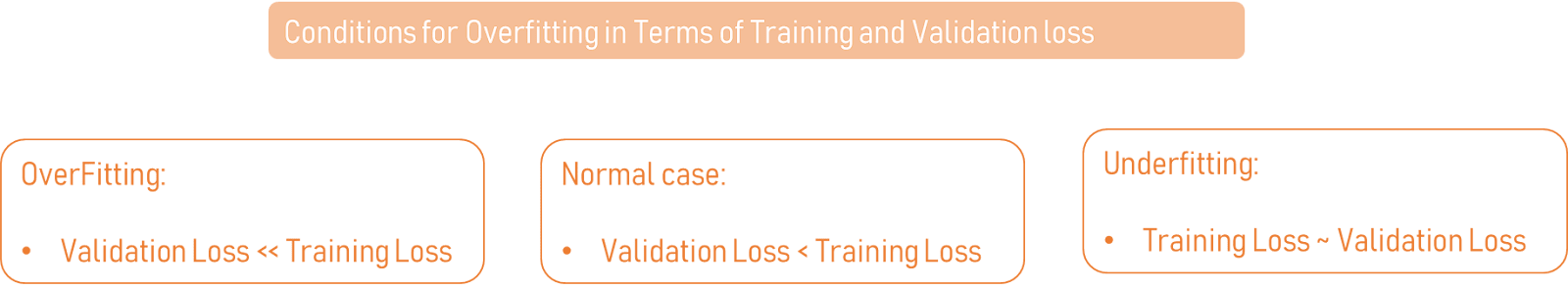
- Overfitting: In this case, the model is too complex and starts to memorize the training data instead of learning the underlying patterns. The model has a low bias, but high variance. The relationship between the validation loss and training loss can be expressed as:
Training Loss << Validation Loss.
- Underfitting: In this case, the model is too simple and is not able to learn the underlying patterns in the data. The model has high bias, but low variance. The relationship between the validation loss and training loss can be expressed as:
Training Loss ~ Validation Loss
- Normal case: In this case, the model is able to learn the underlying patterns in the data and can generalize well to new, unseen data. The model has low bias and low variance. The relationship between the validation loss and training loss can be expressed as:
Training Loss < Validation Loss
Ok, let’s translate the above three points (regarding checkpointing the model) into code. You just need to modify the 4th and 5th chunk of your code i.e., Train the Model and Test the Model code.
epochs = 100
best_loss = float('inf')

# Define checkpoint filename
checkpoint_filename = 'checkpoint.pth.tar'

# Load previous checkpoint if available
if os.path.isfile(checkpoint_filename):
    checkpoint = torch.load(checkpoint_filename)
    start_epoch = checkpoint['epoch']
    best_loss = checkpoint['best_loss']
    model.load_state_dict(checkpoint['state_dict'])
    optimizer.load_state_dict(checkpoint['optimizer'])
    print("Loaded checkpoint '{}' (epoch {})".format(checkpoint_filename, start_epoch))
else:
    start_epoch = 0


for epoch in range(start_epoch, epochs):
    ...
    # Save checkpoint if validation loss is improving
    if val_loss < best_loss:
        best_loss = val_loss
        torch.save({'epoch': epoch+1, 'best_loss': best_loss, 'state_dict': model.state_dict(), 'optimizer': optimizer.state_dict()}, 'best.pth.tar')
        print("Best model so far - saved as 'best.pth.tar'")
    else:
        print("Validation loss did not improve")

    # Save checkpoint at end of epoch
    torch.save({'epoch': epoch+1, 'best_loss': best_loss, 'state_dict': model.state_dict(), 'optimizer': optimizer.state_dict()}, checkpoint_filename)

# Save final model
final_model_filename = 'final_model.pth'
torch.save(model.state_dict(), final_model_filename)
def test_model(model, test_dl):
    # make sure no gradient accumulations happen during forward pass
    with torch.no_grad():
        # list to collect losses across batches for one epoch
        test_losses = []
        for xb, yb in test_dl:
            # forward pass with no gradient accumulations
            pred = model(xb)
            # loss computation per batch
            loss_per_batch = loss_fn(pred, yb)
            test_losses.append(loss_per_batch)
        # print the overall loss
        print('Test Loss: {:.4f}'.format(torch.tensor(test_losses).mean()))

# Load best-saved model for evaluation
if os.path.isfile('best.pth.tar'):
    checkpoint = torch.load('best.pth.tar')
    model.load_state_dict(checkpoint['state_dict'])
    print("Loaded best model checkpoint")

# Evaluate the test dataset against model with best validation loss
test_model(model, test_dl)

# Load final model for evaluation
final_model_filename = 'final_model.pth'
if os.path.isfile(final_model_filename):
    model.load_state_dict(torch.load(final_model_filename))
    print("Loaded final model")
else:
    print("No final model found")

# Evaluate the test dataset against the finally saved model
test_model(model, test_dl)
Go through the code, you can observe all three points we’ve discussed above.
Live Tracking the metrics
Haven’t you felt curious seeing your model’s progress through live updating graphs? Well, I have searched for a lot of libraries for this and found livelossplot but it didn’t offer custom legends options to add. Finally, I’ve used hiddenlayer package which really offered some customization for this.
In summary, we’re going to do two things:
- Tack the validation and training loss plot live
- Add the graphs to the Tensorboard
Note that although you can live to track the progress even with Tensorboard but isn’t possible in Google Colab and is possible in your local computer (since you can run it in localhost:6006 in your command prompt)
Here’s the code you need to add to your Train the Model code.
import os
import hiddenlayer as hl

history1 = hl.History()
history2 = hl.History()
canvas1 = hl.Canvas()

def track_metrics(train_loss, val_loss, epoch):
    # print val and train loss for each epoch
    print('Epoch [{}/{}], Loss: {:.4f}, Val Loss: {:.4f}'.format(epoch+1, epochs, train_loss, val_loss))
    # plot the graphs of train and val loss to tensorboard
    writer.add_scalars("loss", {'train_loss': train_loss, 'val_loss': val_loss}, epoch)

    history1.log(epoch, loss=train_loss)
    history2.log(epoch, loss=val_loss)
    # live plot the train and val loss metrics
    canvas1.draw_plot([history1["loss"], history2["loss"]],
                              labels=["Training Loss", "Validation loss"])
...

for epoch in range(start_epoch, epochs):
    ...
    track_metrics(train_loss, val_loss, epoch)
Run Tensorboard in Google Colab
%reload_ext tensorboard
%tensorboard --logdir=runs
Note on Tensorboard:
Tensorboard offers a lot of options for you to visualize your neural network model. But in this one, we’ve just used it to plot metrics and visualize the model. You can also plot the weights and biases of our model, pr curves, and so on… Here’s the PyTorch official guide for using Tensorborad for you to know more about it.
Conclusion
I know that’s a lot of code mixed with a handful of paragraphs and illustrations. So, here’s the Google Colab code for you to see the entire picture and experiment along. By the way, if you just skimmed through the blog, you might feel PyTorch is not for you. But once you put in enough concentration, then you will definitely find PyTorch is really the one for you rather than going through Abstracted Keras and difficult-to-comprehend customized Tensorflow.